In-Class

Coding Practice

Code 13.1: Predator-Prey Update

We will write a Python module to simulate and visualize population dynamics of a predator-prey system

\[\begin{split} \begin{align*} \Delta N &= r N \left(1 - \frac{N}{K}\right) - a P \frac{N}{N + D}\\ \Delta P &= s P \left(1 - \frac{mP}{N}\right) \end{align*} \end{split}\]

with the parameters \(r\), \(K\), \(a\), \(D\), \(s\), and \(m\). Here, \(N\) and \(P\) are the population sizes of the prey and predator, respectively, and \(\Delta N\) and \(\Delta P\) are the changes in the population sizes per unit time.

We will test the code using the parameters \(r=0.16\), \(K=2400\), \(a=5\), \(D=1000\), \(s=0.01\), and \(m=2\), with the initial population sizes \(N_0=120\) and \(P_0=40\). You can assume that the population sizes are in thousands, and that the time unit is one week.

Explanation of the model

Here is an explanation of the model, but you don’t need to read it to complete the exercise.

The model attempts to describe the dynamics of a biological system in which two species interact, one as a predator (fox) and the other as prey (rabbit). According to the model, in absence of the predator, the prey population grows with the growth constant \(r\) and carrying capacity \(K\). But prey population is subject to predation. If the pray population is abundant, each predator consumes \(k\) prays, while \(D\) is the number of prays required for half-maximal predation. The predator population grows with the growth constant \(s\), and carrying capacity proportional to the prey population, where \(m\) is the number of prays to carry one predator.

Our goal is to define a class PredatorPrey, where object of this class store the parameters of the model. The class should have a method which updates the population sizes according to the models equations.

Start by defining the class PredatorPrey and the __init__ method which initializes the six attributes of the class. Make also a __str__ method which returns a string with the parameters of the model.

Check

At this point, you should be able to achieve the behavior similar to below, but you can choose to construct the string with the parameters differently.

>>> model = PredatorPrey(0.16, 2400, 5, 1000, 0.01, 2)
>>> print(model)
r:0.16, K:2400, k:5, D:1000, s:0.01, m:2

Now we want to write the method update which given the population sizes of the prey and predator returns the updated population sizes. The method should, apart from self, take two arguments N and P which are the population sizes. Inside the method calculate the values of \(\Delta N\) and \(\Delta P\) and return the tuple with \(N + \Delta N\) and \(P + \Delta P\).

Check

At this point, you should be able to achieve the behavior similar to below.

>>> model = PredatorPrey(0.16, 2400, 5, 1000, 0.01, 2)
>>> model.update(120, 40)
(116.81142857142856, 40.13333333333333)

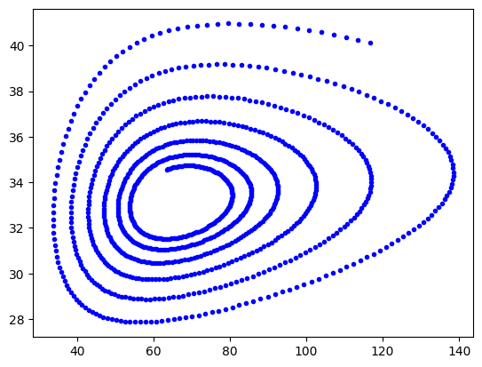
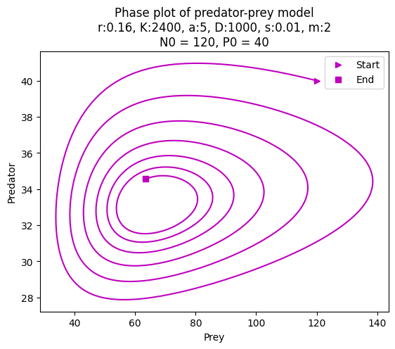
Now we can use the class for the first attempt to simulate the population dynamics. Starting with the parameters as in the check above, write a for-loop which updates the population sizes for 1000 iterations. In the loop. plot the population sizes of the prey and predator as a point in the predator-pray plane using the Matplotlib library. Your plot should look similar to the one below.

Hint

For update, use can use tuple unpacking N, P = model.update(N, P). For plotting, use plt.plot(N, P, 'b.').

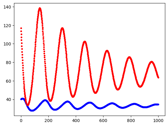
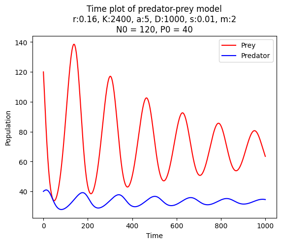
Try also plotting the time evolution of the population sizes of the prey and predator. Your plot should look similar to the one below.

Hint

Plot predator and pray against the iterator of the for-loop. Use different colors for the two species, for example, plt.plot(i, N, 'r.') and plt.plot(i, P, 'b.').

Code 13.2: Predator-Prey Evolution

We would like to plot the evolution as a curve, and not as points. To do this, we need to store the population sizes in a list.

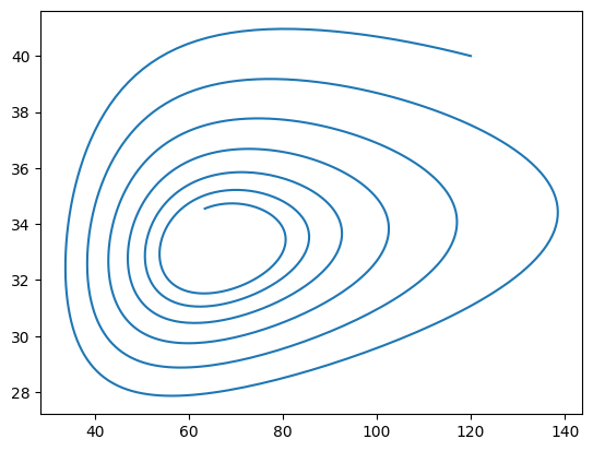
Modify your code such that you before the loop define two lists N_values and P_values, which initially only contain the initial population sizes. In the loop, append the updated population sizes to the lists. After the loop, plot the lists using the Matplotlib library. Your plot should look similar to the one below.

Hint

For a compact code, you can use tuple unpacking when defining lists N_values, P_values = [N], [P]. Make sure to plot outside the body of the for-loop.

Instead of looping in the main code, write a method evolve in the class PredatorPrey. The method should take the initial population sizes and the number of iterations as arguments. The method should return the lists N_values and P_values.

Check

At this point, running the code block below should produce the plot similar to the one above.

model = PredatorPrey(0.16, 2400, 5, 1000, 0.01, 2)
N_values, P_values = model.evolve(120, 40, 1000)
plt.plot(N_values, P_values)
plt.show()

Instead of plotting in the main code, define a method plot_evolution in the class PredatorPrey. The method should take the initial population sizes and the number of iterations as arguments. The method should produce two plots. The firs is a phase plot where prey and predator populations are plotted against each other. The second is a time plot where prey and predator populations are plotted against the iteration number. Add as many information to the plots as you find useful: labels, titles, legends, etc. The code below shows how the method should be used, and you can look at the produced plots for inspiration.

model = PredatorPrey(0.16, 2400, 5, 1000, 0.01, 2)
model.plot_evolution(120, 40, 1000)

Hint

To make a title with multiple lines, use \n in the string, for example, plt.title('Predator-Prey Model\nPhase Plot').

Code 13.3: Predator-Prey Module

Once you have a well-working class, divide your code in two python files. Name one file predator_prey.py and keep only class definition in it. This is the module we produced. You need to import Matplotlib in the module, since you use it in the method which plots the evolution. Name the other file predator_prey_simulation.py. This is the main script. In the main script, import the class from the module. Use the class to produce the plots as in the previous exercise.

If you have done everything correctly, your main script need only to contain three lines of code.

Check

At this point, the code below executed from the main script should produce the plots.

from predator_prey import PredatorPrey as PP

model = PP(0.16, 2400, 5, 1000, 0.01, 2)
model.plot_evolution(120, 40, 1000)

By separating your code in the module and the script, you can reuse the module in the other scripts, and your script is simpler and easier to read.

Problem Solving

Problem 13.4: Allee Effect Analysis

You should write a Python module which can be used to analyze the Allee effect in a population. The Alle effect is modeled using the differential equation

\[ \frac{\mathrm{d}N}{\mathrm{d}t} = r N \left(1 - \frac{N}{K}\right) \left(\frac{N}{A} - 1\right) \]

where \(N\) is the population size, \(r\) is the growth rate, \(K\) is the carrying capacity, and \(A<K\) is the Allee threshold.

Explanation of the model

Here is an explanation of the model, but you don’t need to read it to complete the exercise.

The model attempts to describe the dynamics of a biological system in which the population growth rate decreases at low population sizes, and reaches saturation at hight population sizes. The factor \(rN\) describes exponential growth in the absence of other effects. The factor \((1-N/K)\) describes saturation: if the population size is close to carrying capacity \(K\), this factor is close to zero, and the growth rate is small. If the population is larger than \(K\), this factor is negative, and the growth rate is negative. The population will therefore stabilize at \(K\). The factor \((N/A - 1)\) describes the Allee effect: if the population size is below the Allee threshold \(A\), this factor is negative, and the growth rate is negative. This means that the population size decreases if it is below the Allee threshold.

You should make a class AlleeEffect which has the following methods:

• __init__ which initializes the attributes of the class, which are the growth rate \(r\), the carrying capacity \(K\), and the Allee threshold \(A\).

• __str__ which returns a string with the parameters of the model. You can choose the format of the string.

• update which given the population size \(N\) and the time step \(\Delta t\) returns the updated population size \(N + \frac{\mathrm{d}N}{\mathrm{d}t}\Delta t\).

• evolve which given the initial population size, the length of the time interval, and the time step \(\Delta t\) returns the list of time steps and the list of population sizes. The list of time steps should start with 0, increase by \(\Delta t\), and end with the length of the time interval. The list of population sizes should start with the initial population size and be updated using the update method.

• plot_evolutions which given the list of initial population sizes, the length of the time interval, and the time step \(\Delta t\), produces a plot of the population sizes as a function of time. The plot should contain as many curves as there are initial population sizes.

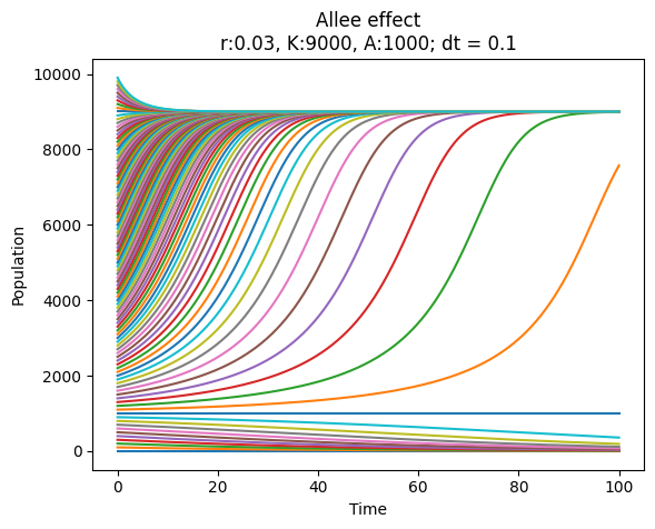
Place the class in the module allee_effect.py and write a script allee_effect_simulation.py which imports the class and uses it to produce a plot of the population size as a function of time. Use the parameters \(r=0.03\), \(K=9000\), and \(A=1000\), a number of initial population size in a interval between 0 and 10000, the time step \(\Delta t=0.1\) and the length of the time interval \(T=100\).

Look at the code below and the plot for the desired behavior of the script.

from alle_effect import AlleeEffect as AE
model = AE(0.03, 9000, 1000)
model.plot_evolutions(list(range(0, 10000, 100)), 100, 0.1)